Examples
These examples and the input data for these examples can found in the examples/ or test_data/ folders of the github repository.
Basic Examples
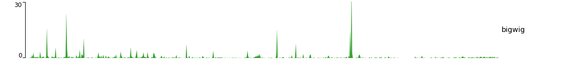
A minimal example of a configuration file with a single bigwig track looks like this:
[bigwig file test]
file = bigwig.bw
# height of the track in cm (optional value)
height = 4
title = bigwig
min_value = 0
max_value = 30
$ pyGenomeTracks --tracks bigwig_track.ini --region X:2,500,000-3,000,000 -o bigwig.png
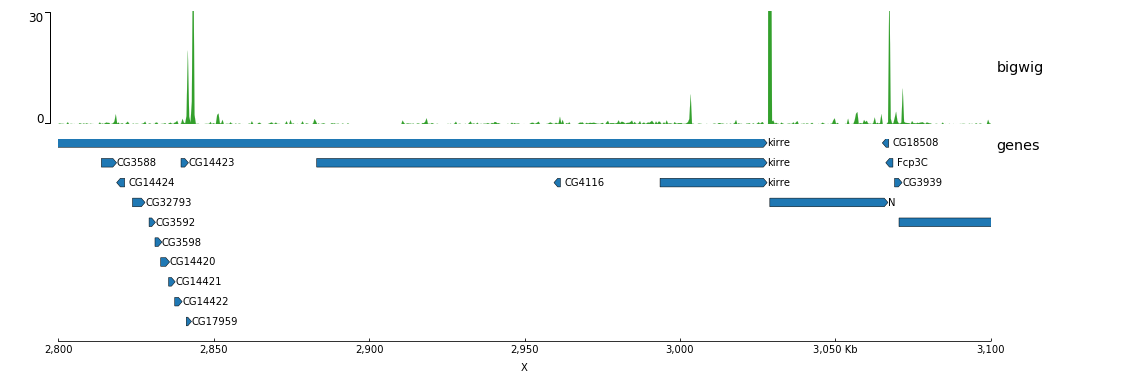
Now, let’s add the genomic location and some genes:
[bigwig file test]
file = bigwig.bw
# height of the track in cm (optional value)
height = 4
title = bigwig
min_value = 0
max_value = 30

[spacer]
# this simply adds an small space between the two tracks.

[genes]
file = genes.bed.gz
height = 7
title = genes
fontsize = 10
file_type = bed
gene_rows = 10

[x-axis]
fontsize=10
$ pyGenomeTracks --tracks bigwig_with_genes.ini --region X:2,800,000-3,100,000 -o bigwig_with_genes.png
Now, we will add some vertical lines across all tracks. The vertical lines should be in a bed format.
[bigwig file test]
file = bigwig.bw
# height of the track in cm (optional value)
height = 4
title = bigwig
min_value = 0
max_value = 30

[spacer]
# this simply adds an small space between the two tracks.

[genes]
file = genes.bed.gz
height = 7
title = genes
fontsize = 10
file_type = bed
gene_rows = 10

[x-axis]
fontsize=10

[vlines]
file = domains.bed
type = vlines
$ pyGenomeTracks --tracks bigwig_with_genes_and_vlines.ini --region X:2,800,000-3,100,000 -o bigwig_with_genes_and_vlines.png

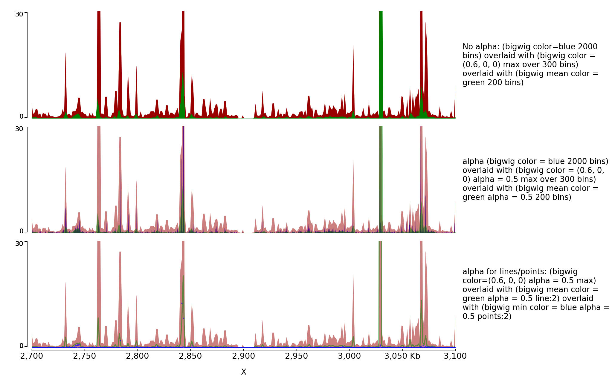
You can also overlay bigwig with or without transparency.
[test bigwig]
file = bigwig2_X_2.5e6_3.5e6.bw
color = blue
height = 7
title = No alpha: (bigwig color=blue 2000 bins) overlaid with (bigwig color = (0.6, 0, 0) max over 300 bins) overlaid with (bigwig mean color = green 200 bins)
number_of_bins = 2000
min_value = 0
max_value = 30

[test bigwig max]
file = bigwig2_X_2.5e6_3.5e6.bw
color = (0.6, 0, 0)
summary_method = max
number_of_bins = 300
overlay_previous = share-y

[test bigwig mean]
file = bigwig2_X_2.5e6_3.5e6.bw
color = green
type = fill
number_of_bins = 200
overlay_previous = share-y

[spacer]

[test bigwig]
file = bigwig2_X_2.5e6_3.5e6.bw
color = blue
height = 7
title = alpha (bigwig color = blue 2000 bins) overlaid with (bigwig color = (0.6, 0, 0) alpha = 0.5 max over 300 bins) overlaid with (bigwig mean color = green alpha = 0.5 200 bins)
number_of_bins = 2000
min_value = 0
max_value = 30

[test bigwig max]
file = bigwig2_X_2.5e6_3.5e6.bw
color = (0.6, 0, 0)
alpha = 0.5
summary_method = max
number_of_bins = 300
overlay_previous = share-y

[test bigwig mean]
file = bigwig2_X_2.5e6_3.5e6.bw
color = green
alpha = 0.5
type = fill
number_of_bins = 200
overlay_previous = share-y

[spacer]

[test bigwig]
file = bigwig2_X_2.5e6_3.5e6.bw
height = 7
title = alpha for lines/points: (bigwig color=(0.6, 0, 0) alpha = 0.5 max) overlaid with (bigwig mean color = green alpha = 0.5 line:2) overlaid with (bigwig min color = blue alpha = 0.5 points:2)
color = (0.6, 0, 0)
alpha = 0.5
summary_method = max
number_of_bins = 300
min_value = 0
max_value = 30

[test bigwig mean]
file = bigwig2_X_2.5e6_3.5e6.bw
color = green
type = line:2
alpha = 0.5
summary_method = mean
number_of_bins = 300
overlay_previous = share-y

[test bigwig min]
file = bigwig2_X_2.5e6_3.5e6.bw
color = blue
summary_method = min
number_of_bins = 1000
type = points:3
alpha = 0.5
overlay_previous = share-y

[x-axis]
$ pyGenomeTracks --tracks alpha.ini --region X:2700000-3100000 --trackLabelFraction 0.2 --dpi 130 -o master_alpha.png
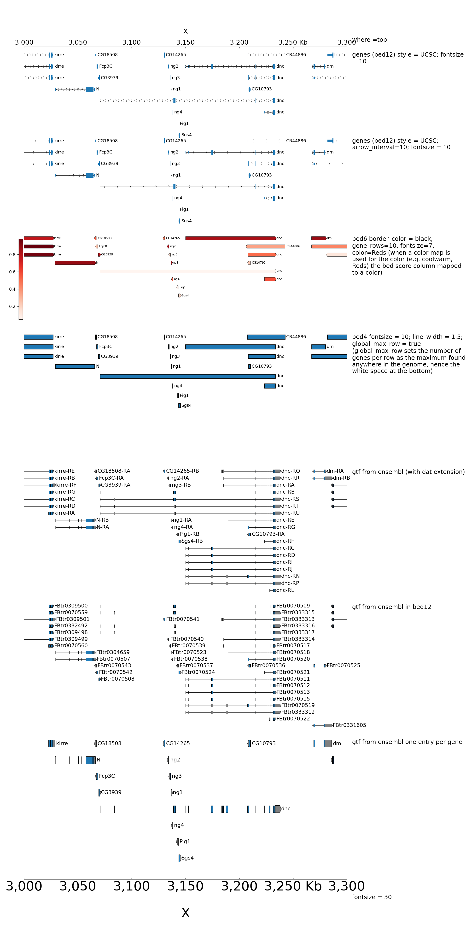
Examples with bed and gtf
Here is an example to explain the parameters for bed and gtf:
[x-axis]
where = top
title = where =top

[spacer]
height = 0.05

[genes 2]
file = dm3_genes.bed.gz
height = 7
title = genes (bed12) style = UCSC; fontsize = 10
style = UCSC
fontsize = 10

[genes 2bis]
file = dm3_genes.bed.gz
height = 7
title = genes (bed12) style = UCSC; arrow_interval=10; fontsize = 10
style = UCSC
arrow_interval = 10
fontsize = 10

[spacer]
height = 1

[test bed6]
file = dm3_genes.bed6.gz
height = 7
title = bed6 border_color = black; gene_rows=10; fontsize=7; color=Reds (when a color map is used for the color (e.g. coolwarm, Reds) the bed score column mapped to a color)
fontsize = 7
file_type = bed
color = Reds
border_color = black
gene_rows = 10

[spacer]
height = 1

[test bed4]
file = dm3_genes.bed4.gz
height = 10
title = bed4 fontsize = 10; line_width = 1.5; global_max_row = true (global_max_row sets the number of genes per row as the maximum found anywhere in the genome, hence the white space at the bottom)
fontsize = 10
file_type = bed
global_max_row = true
line_width = 1.5

[spacer]
height = 1

[test gtf]
file = dm3_subset_BDGP5.78_gtf.dat
height = 10
title = gtf from ensembl (with dat extension)
fontsize = 12
file_type = gtf

[spacer]
height = 1

[test bed]
file = dm3_subset_BDGP5.78_asbed_sorted.bed.gz
height = 10
title = gtf from ensembl in bed12
fontsize = 12
file_type = bed

[spacer]
height = 1

[test gtf collapsed]
file = dm3_subset_BDGP5.78.gtf.gz
height = 10
title = gtf from ensembl one entry per gene
merge_transcripts = true
prefered_name = gene_name
fontsize = 12
file_type = gtf

[spacer]
height = 1

[x-axis]
fontsize = 30
title = fontsize = 30
$ pyGenomeTracks --tracks bed_and_gtf_tracks.ini --region X:3000000-3300000 --trackLabelFraction 0.2 --width 38 --dpi 130 -o master_bed_and_gtf.png
By default, when bed are displayed and interval are stranded, the arrowhead which indicates the direction is plotted outside of the interval. Here is an example to show how to put it inside:
[x-axis]
where = top
title = where =top

[spacer]
height = 0.05

[genes 2]
file = dm3_genes.bed.gz
height = 3
title = genes (bed12) style = UCSC; fontsize = 10
style = UCSC
fontsize = 10

[genes 2bis]
file = dm3_genes.bed.gz
height = 3
title = genes (bed12) style = UCSC; arrow_interval=10; fontsize = 10
style = UCSC
arrow_interval = 10
fontsize = 10

[spacer]
height = 1

[test bed6]
file = dm3_genes.bed6.gz
height = 3
title = bed6 border_color = black; fontsize=8; color=red
fontsize = 8
file_type = bed
color = red
border_color = black

[spacer]
height = 1

[test bed6 arrowhead_included]
file = dm3_genes.bed6.gz
height = 3
title = bed6 border_color = black; fontsize=8; color=red; arrowhead_included = true
fontsize = 8
file_type = bed
color = red
border_color = black
arrowhead_included = true

[spacer]
height = 1

[test bed4]
file = dm3_genes.bed4.gz
height = 3
title = bed4 fontsize = 10; line_width = 1.5
fontsize = 10
file_type = bed
line_width = 1.5

[spacer]
height = 1

[test bed]
file = dm3_subset_BDGP5.78_asbed_sorted.bed.gz
height = 8
title = gtf from ensembl in bed12
fontsize = 12
file_type = bed

[spacer]
height = 1

[test bed]
file = dm3_subset_BDGP5.78_asbed_sorted.bed.gz
height = 8
title = gtf from ensembl in bed12; arrowhead_included = true
fontsize = 12
file_type = bed
arrowhead_included = true

[spacer]
height = 1

[x-axis]
fontsize = 30
title = fontsize = 30

[vlines]
type = vlines
file = dm3_genes.bed4.gz
line_style = dotted

[second_vlines]
type = vlines
file = dm3_genes_end.bed
line_width = 1
color = orange
zorder = -100
$ pyGenomeTracks --tracks bed_arrow_tracks.ini --region X:3130000-3140000 --trackLabelFraction 0.2 --width 38 --dpi 130 -o master_bed_arrow_zoom.png
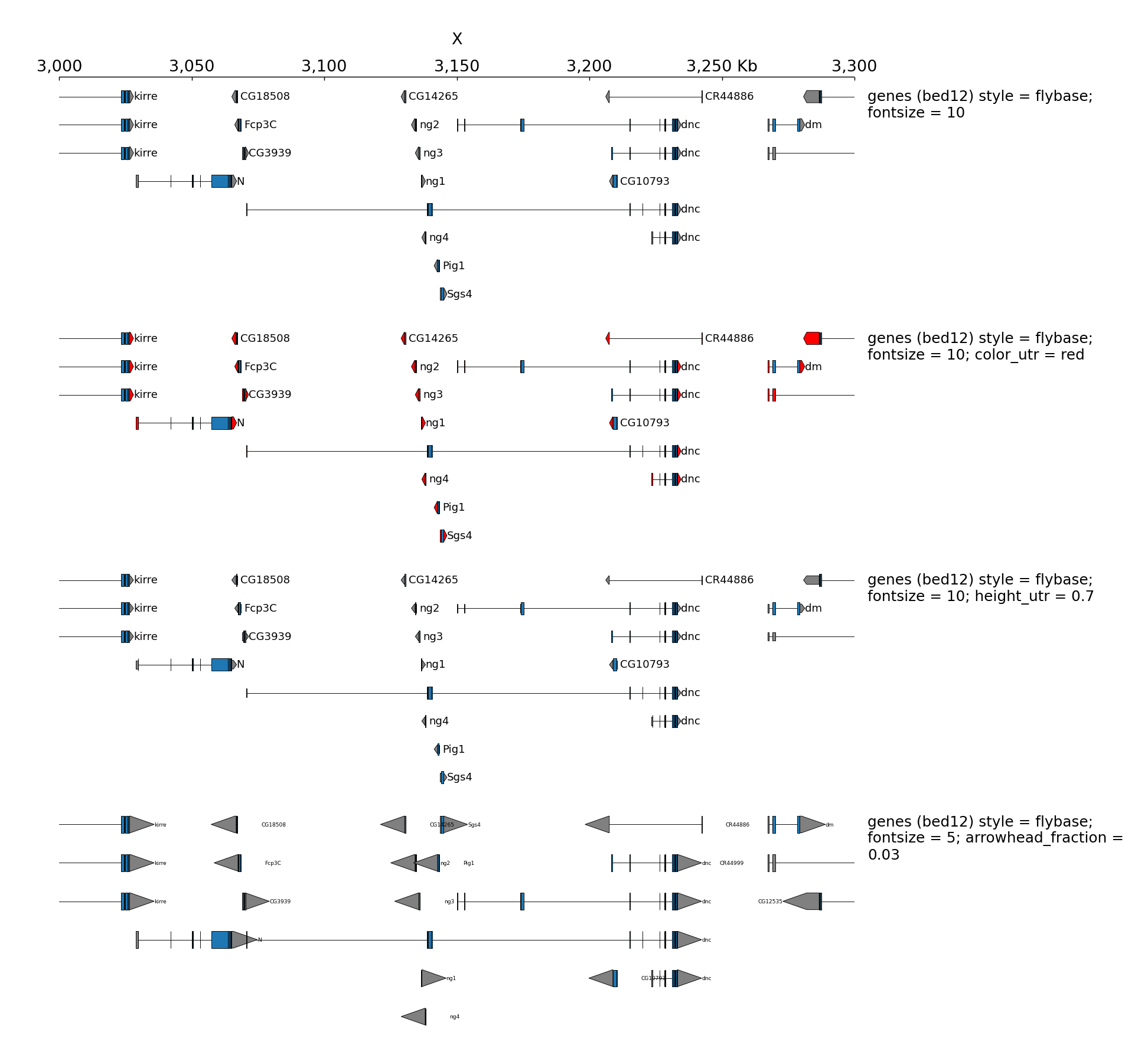
When genes are displayed with the default style (flybase), the color and the height of UTR can be set:
[x-axis]
where = top

[spacer]
height = 0.05

[genes 0]
file = dm3_genes.bed.gz
height = 7
title = genes (bed12) style = flybase; fontsize = 10
style = flybase
fontsize = 10

[spacer]
height = 1

[genes 1]
file = dm3_genes.bed.gz
height = 7
title = genes (bed12) style = flybase; fontsize = 10; color_utr = red
style = flybase
fontsize = 10
color_utr = red

[spacer]
height = 1

[genes 2]
file = dm3_genes.bed.gz
height = 7
title = genes (bed12) style = flybase; fontsize = 10; height_utr = 0.7
style = flybase
fontsize = 10
height_utr = 0.7

[spacer]
height = 1

[genes 3]
file = dm3_genes.bed.gz
height = 7
title = genes (bed12) style = flybase; fontsize = 5; arrowhead_fraction = 0.03
style = flybase
fontsize = 5
arrowhead_fraction = 0.03
all_labels_inside = true
$ pyGenomeTracks --tracks bed_flybase_tracks.ini --region X:3000000-3300000 --trackLabelFraction 0.2 --width 38 --dpi 130 -o master_bed_flybase.png
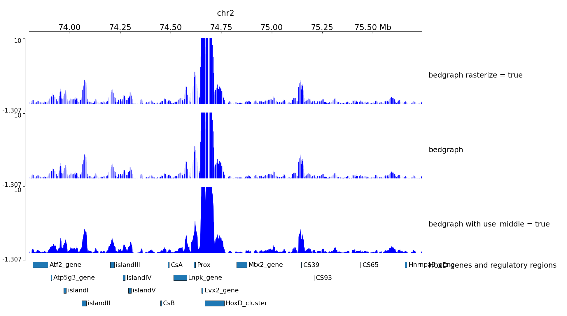
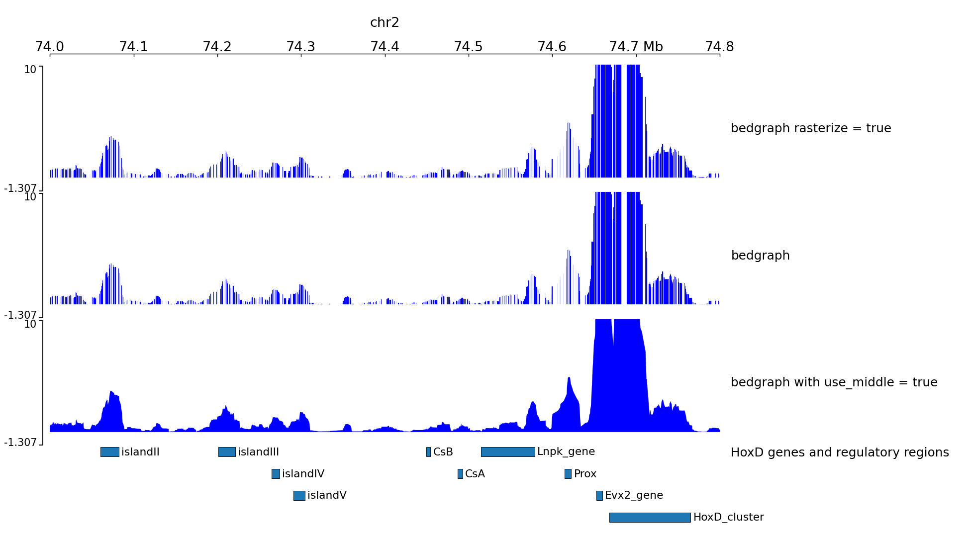
Examples with 4C-seq
The output file of some 4C-seq pipeline are bedgraph where the coordinates are the coordinates of the fragment. In these cases, it can be interesting to remove the regions absent from the file and just link the middle of the fragments together instead of plotting a rectangle for each fragment. Here is an example of the option use_middle
[x-axis]
where = top

[spacer]
height = 0.05

[test bedgraph]
file = GSM3182416_E12DHL_WT_Hoxd11vp.bedgraph.gz
color = blue
height = 5
title = bedgraph rasterize = true
rasterize = true
max_value = 10

[test bedgraph]
file = GSM3182416_E12DHL_WT_Hoxd11vp.bedgraph.gz
color = blue
height = 5
title = bedgraph
max_value = 10

[test bedgraph use middle]
file = GSM3182416_E12DHL_WT_Hoxd11vp.bedgraph.gz
color = blue
height = 5
title = bedgraph with use_middle = true
max_value = 10
use_middle = true

[genes]
file = HoxD_cluster_regulatory_regions_mm10.bed
height = 3
title = HoxD genes and regulatory regions
We can generate two zooms using a bed instead of regions:
track type=bed name=regions_to_plot
chr2	73800000	75744000
chr2	74000000	74800000
$ pyGenomeTracks --tracks bedgraph_useMid.ini --BED regions_imbricated_chr2.bed --trackLabelFraction 0.2 --width 38 --dpi 130 -o master_bedgraph_useMid.png
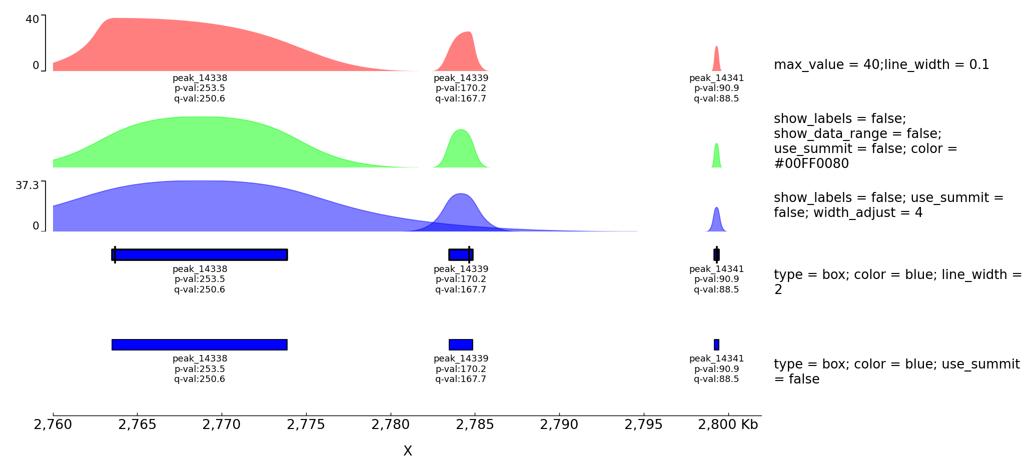
Examples with peaks
pyGenomeTracks has an option to plot peaks using MACS2 narrowPeak format.
The following is an example of the output in which the peak shape is drawn based on the start, end, summit and height of the peak.
[narrow]
file = test2.narrowPeak
height = 4
max_value = 40
line_width = 0.1
title = max_value = 40;line_width = 0.1

[narrow 2]
file = test2.narrowPeak
height = 2
show_labels = false
show_data_range =  false
color = #00FF0080
use_summit = false
title = show_labels = false; show_data_range = false; use_summit = false; color = #00FF0080

[spacer]

[narrow 3]
file = test2.narrowPeak
height = 2
show_labels = false
color = #0000FF80
use_summit = false
width_adjust = 4
title = show_labels = false; use_summit = false; width_adjust = 4

[spacer]

[narrow 4]
file = test2.narrowPeak
height = 3
type = box
color = blue
line_width = 2
title = type = box; color = blue; line_width = 2

[spacer]

[narrow 5]
file = test2.narrowPeak
height = 3
type = box
color = blue
use_summit = false
title = type = box; color = blue; use_summit = false

[x-axis]
$ pyGenomeTracks --tracks narrow_peak2.ini --region X:2760000-2802000 --trackLabelFraction 0.2 --dpi 130 -o master_narrowPeak2.png
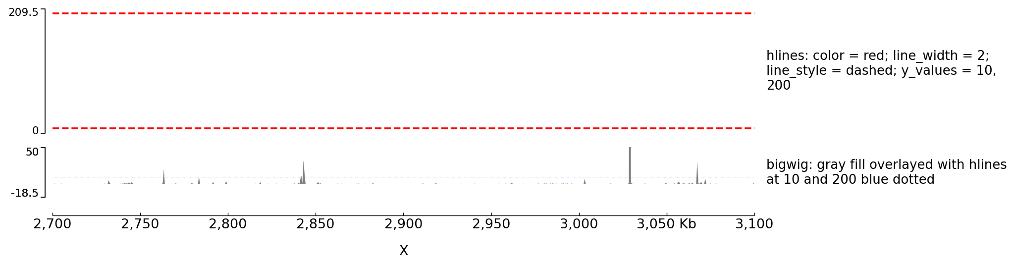
Example with horizontal lines
[test hlines]
color = red
line_width = 2
line_style = dashed
y_values = 10, 200
min_value = 0
show_data_range = true
height = 5
title = hlines: color = red; line_width = 2; line_style = dashed; y_values = 10, 200
file_type = hlines

[spacer]

[test bigwig fill]
file = bigwig2_X_2.5e6_3.5e6.bw
color = gray
height = 2
type = fill
title = bigwig: gray fill overlayed with hlines at 10 and 200 blue dotted
max_value = 50

[test hlines ovelayed]
color = blue
line_style = dotted
y_values = 10, 200
overlay_previous = share-y
file_type = hlines

[spacer]

[x-axis]
$ pyGenomeTracks --tracks hlines.ini --region X:2700000-3100000 --trackLabelFraction 0.2 --dpi 130 -o master_hlines.png
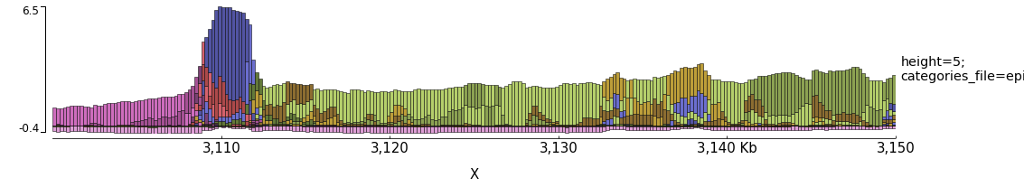
Examples with Epilogos
pyGenomeTracks can be used to visualize epigenetic states (for example from chromHMM) as epilogos. For more information see: https://epilogos.altiusinstitute.org/
To plot epilogos a qcat file is needed. This file can be crated using the epilogos software (https://github.com/Altius/epilogos).
An example track file for epilogos looks like:
[epilogos]
file = epilog.qcat.bgz
height = 5
title = height=5; categories_file=epilog_cats.json

[x-axis]
$ pyGenomeTracks --tracks epilogos_track.ini --region X:3100000-3150000 -o epilogos_track.png
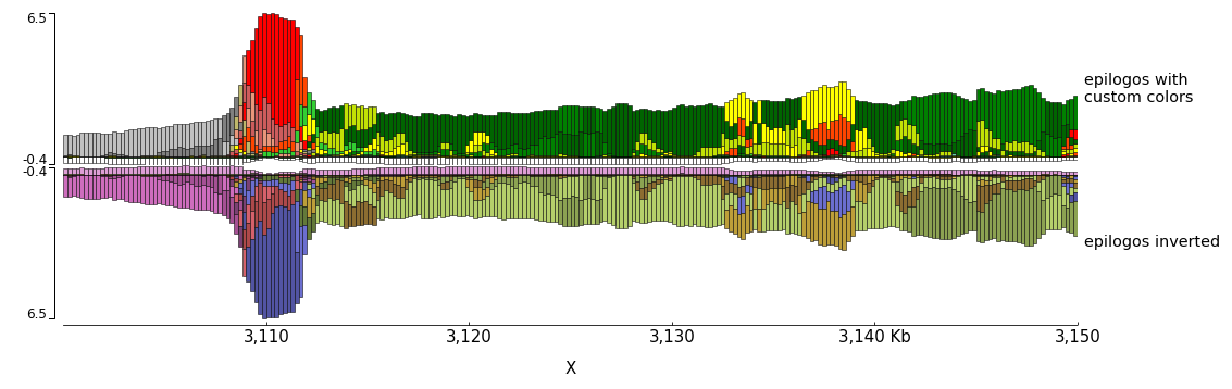
The color of the bars can be set by using a json file. The structure of the file is like this
{
"categories":{
          "1":["Active TSS","#ff0000"],
          "2":["Flanking Active TSS","#ff4500"],
          "3":["Transcr at gene 5\" and 3\"","#32cd32"],
          "4":["Strong transcription","#008000"],
          "5":["Weak transcription","#006400"],
          "6":["Genic enhancers","#c2e105"],
          "7":["Enhancers","#ffff00"],
          "8":["ZNF genes & repeats","#66cdaa"],
          "9":["Heterochromatin","#8a91d0"],
          "10":["Bivalent/Poised TSS","#cd5c5c"],
          "11":["Flanking Bivalent TSS/Enh","#e9967a"],
          "12":["Bivalent Enhancer","#bdb76b"],
          "13":["Repressed PolyComb","#808080"],
          "14":["Weak Repressed PolyComb","#c0c0c0"],
          "15":["Quiescent/Low","#ffffff"]
	}
}
In the following examples the top epilogo has the custom colors and the one below is shown inverted.
[epilogos]
file = epilog.qcat.bgz
height = 5
title = epilogos with custom colors
categories_file = epilog_cats.json

[epilogos inverted]
file = epilog.qcat.bgz
height = 5
title = epilogos inverted
orientation = inverted

[x-axis]
$ pyGenomeTracks --tracks epilogos_track2.ini --region X:3100000-3150000 -o epilogos_track2.png
Examples with multiple options
A comprehensive example of pyGenomeTracks can be found as part of our automatic testing.
Note, that pyGenomeTracks also allows the combination of multiple tracks into one using the parameter: overlay_previous = yes or overlay_previous = share-y.
In the second option the y-axis of the tracks that overlays is the same as the track being overlay. Multiple tracks can be overlay together.
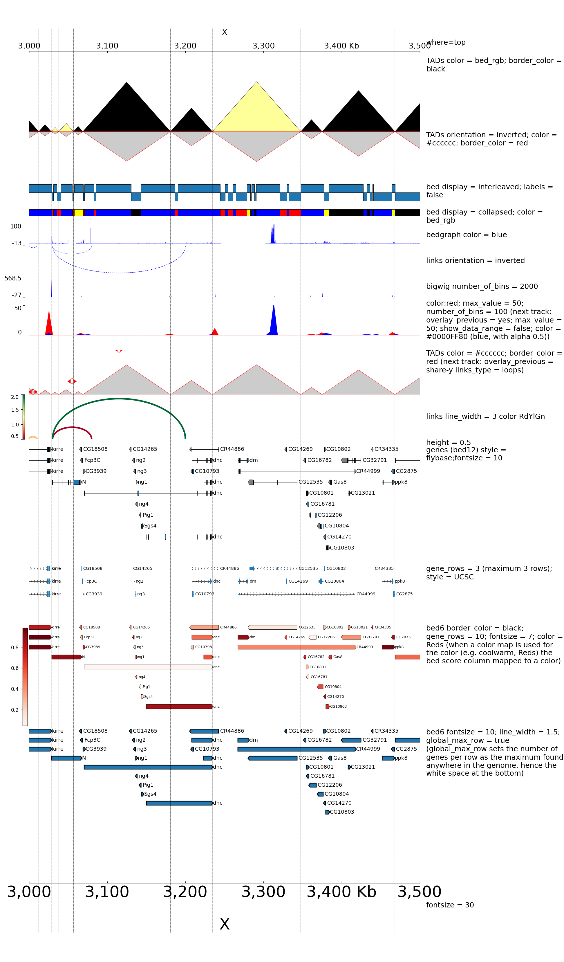
The configuration file for this image is:
[x-axis]
where = top
title = where=top

[spacer]
height = 0.05

[tads]
file = tad_classification.bed
title = TADs color = bed_rgb; border_color = black
file_type = domains
border_color = black
color = bed_rgb
height = 5

[tads 2]
file = tad_classification.bed
title = TADs orientation = inverted; color = #cccccc; border_color = red
file_type = domains
border_color = red
color = #cccccc
orientation = inverted
height = 3

[spacer]
height = 0.5

[tad state]
file = chromatinStates_kc.bed.gz
height = 1.2
title = bed display = interleaved; labels = false
display = interleaved
labels = false

[spacer]
height = 0.5

[tad state]
file = chromatinStates_kc.bed.gz
height = 0.5
title = bed display = collapsed; color = bed_rgb
labels = false
color = bed_rgb
display = collapsed

[spacer]
height = 0.5

[test bedgraph]
file = bedgraph_chrx_2e6_5e6.bg
color = blue
height = 1.5
title = bedgraph color = blue
max_value = 100

[test arcs]
file = test.arcs
title = links orientation = inverted
orientation = inverted
line_style = dashed
height = 2

[test bigwig]
file = bigwig2_X_2.5e6_3.5e6.bw
color = blue
height = 1.5
title = bigwig number_of_bins = 2000
number_of_bins = 2000

[spacer]

[test bigwig overlay]
file = bigwig2_X_2.5e6_3.5e6.bw
color = red
title = color:red; max_value = 50; number_of_bins = 100 (next track: overlay_previous = yes; max_value = 50; show_data_range = false; color = #0000FF80 (blue, with alpha 0.5))
min_value = 0
max_value = 50
height = 2
number_of_bins = 100

[test bigwig overlay]
file = bigwig_chrx_2e6_5e6.bw
color = #0000FF80
title =
min_value = 0
max_value = 50
show_data_range = false
overlay_previous = yes
number_of_bins = 100

[spacer]
height = 1

[tads 3]
file = tad_classification.bed
title = TADs color = #cccccc; border_color = red (next track: overlay_previous = share-y links_type = loops)
file_type = domains
border_color = red
color = #cccccc
height = 3

[test arcs overlay]
file = test.arcs
color = red
line_width = 10
links_type = loops
overlay_previous = share-y

[test arcs]
file = test.arcs
line_width = 3
color = RdYlGn
title = links line_width = 3 color RdYlGn
height = 3

[spacer]
height = 0.5
title = height = 0.5

[genes 2]
file = dm3_genes.bed.gz
height = 7
title = genes (bed12) style = flybase;fontsize = 10
style = flybase
fontsize = 10

[spacer]
height = 1

[test gene rows]
file = dm3_genes.bed.gz
height = 3
title = gene_rows = 3 (maximum 3 rows); style = UCSC
fontsize = 8
style = UCSC
gene_rows = 3

[spacer]
height = 1

[test bed6]
file = dm3_genes.bed6.gz
height = 7
title = bed6 border_color = black; gene_rows = 10; fontsize = 7; color = Reds (when a color map is used for the color (e.g. coolwarm, Reds) the bed score column mapped to a color)
fontsize = 7
file_type = bed
color = Reds
border_color = black
gene_rows = 10

[test bed6]
file = dm3_genes.bed6.gz
height = 10
title = bed6 fontsize = 10; line_width = 1.5; global_max_row = true (global_max_row sets the number of genes per row as the maximum found anywhere in the genome, hence the white space at the bottom)
fontsize = 10
file_type = bed
global_max_row = true
line_width = 1.5

[x-axis]
fontsize = 30
title = fontsize = 30

[vlines]
file = tad_classification.bed
type = vlines
$ pyGenomeTracks --tracks browser_tracks.ini --region X:3000000-3500000 --trackLabelFraction 0.2 --width 38 --dpi 130 -o master_plot.png
Examples with multiple options for bigwig tracks
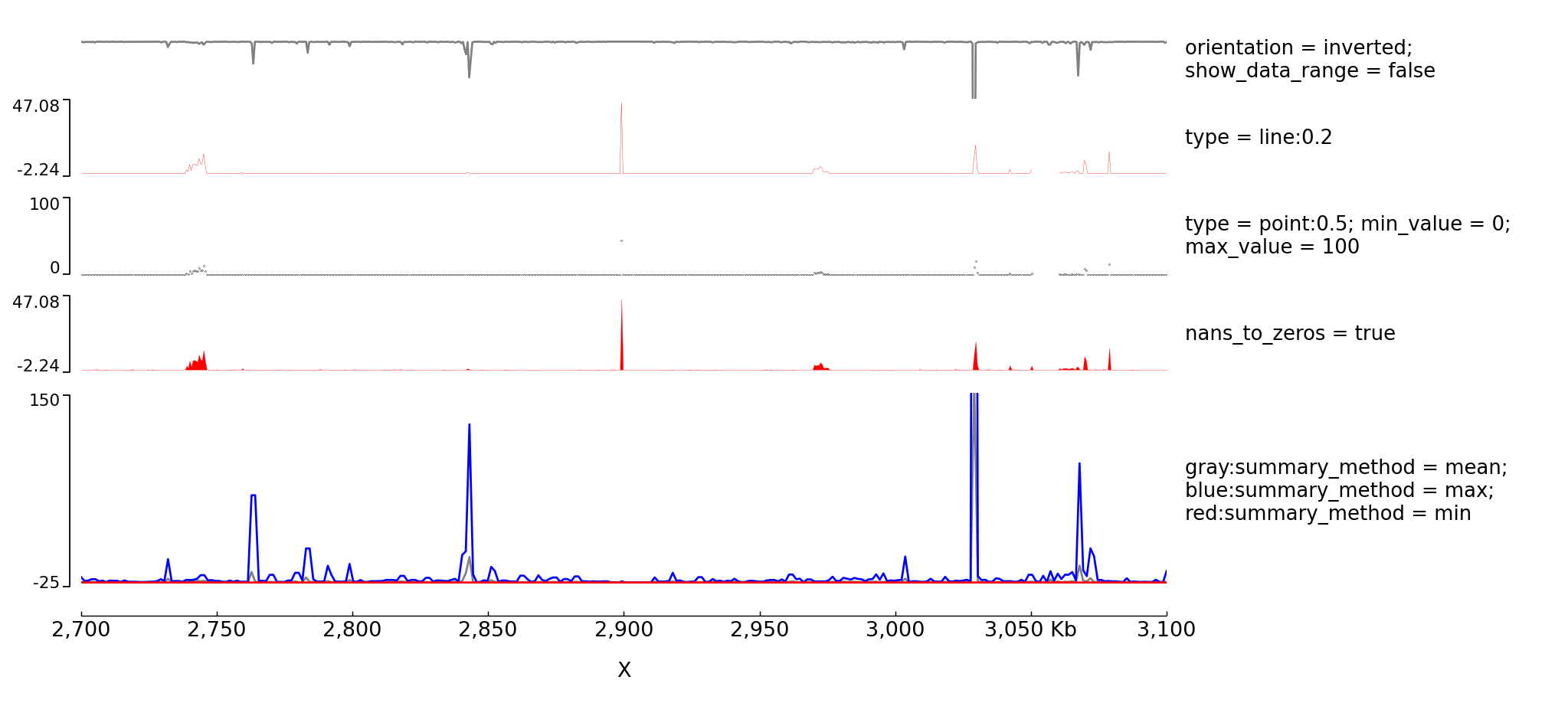
The configuration file for this image is:
[test bigwig lines]
file = bigwig2_X_2.5e6_3.5e6.bw
color = gray
height = 2
type = line
title = orientation = inverted; show_data_range = false
orientation = inverted
show_data_range = false
max_value = 50

[test bigwig lines:0.2]
file = bigwig_chrx_2e6_5e6.bw
color = red
height = 2
type = line:0.2
title = type = line:0.2
min_value = auto
max_value = auto

[spacer]

[test bigwig points]
file = bigwig_chrx_2e6_5e6.bw
color = black
height = 2
min_value = 0
max_value = 100
type = points:0.5
title = type = point:0.5; min_value = 0; max_value = 100

[spacer]

[test bigwig nans to zeros]
file = bigwig_chrx_2e6_5e6.bw
color = red
height = 2
nans_to_zeros = true
title = nans_to_zeros = true

[spacer]

[test bigwig mean]
file = bigwig2_X_2.5e6_3.5e6.bw
color = gray
height = 5
title = gray:summary_method = mean; blue:summary_method = max; red:summary_method = min
type = line
summary_method = mean
max_value = 150
min_value = -5
show_data_range = false
number_of_bins = 300

[test bigwig max]
file = bigwig2_X_2.5e6_3.5e6.bw
#title = test
color = blue
type = line
summary_method = max
max_value = 150
min_value = -15
show_data_range = false
overlay_previous = share-y
number_of_bins = 300

[test bigwig min]
file = bigwig2_X_2.5e6_3.5e6.bw
color = red
type = line
summary_method = min
max_value = 150
min_value = -25
overlay_previous = share-y
number_of_bins = 300

[spacer]

[x-axis]
$ pyGenomeTracks --tracks bigwig.ini --region X:2700000-3100000 --trackLabelFraction 0.2 --dpi 130 -o master_bigwig.png
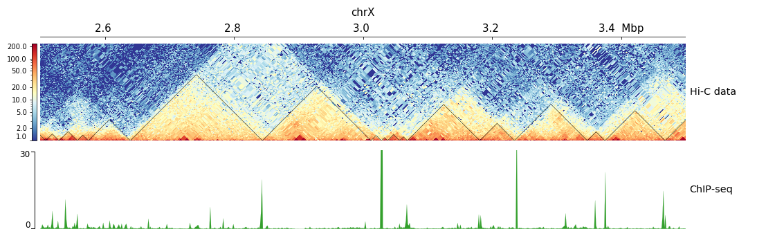
Examples with Hi-C data
The following is an example with Hi-C data overlay with topologically associating domains (TADs) and a bigwig file.
[x-axis]
where = top

[hic matrix]
file = hic_data.h5
title = Hi-C data
# depth is the maximum distance plotted in bp. In Hi-C tracks
# the height of the track is calculated based on the depth such
# that the matrix does not look deformed
depth = 300000
transform = log1p
file_type = hic_matrix

[tads]
file = domains.bed
display = triangles
border_color = black
color = none
# the tads are overlay over the hic-matrix
# the share-y options sets the y-axis to be shared
# between the Hi-C matrix and the TADs.
overlay_previous = share-y

[spacer]

[bigwig file test]
file = bigwig.bw
# height of the track in cm (optional value)
height = 4
title = ChIP-seq
min_value = 0
max_value = 30
$ pyGenomeTracks --tracks hic_track.ini -o hic_track.png --region chrX:2500000-3500000
Here is an example where the height was set or not set and the heatmap was rasterized (default) or not rasterized (the dpi was set very low just to show the impact of the parameter).
[hic matrix]
file = Li_et_al_2015.cool
title = depth = 200000; transform = log1p; min_value = 5; height = 5
depth = 200000
min_value = 5
transform = log1p
file_type = hic_matrix
show_masked_bins = false
height = 5

[hic matrix 2]
file = Li_et_al_2015.h5
title = same but orientation=inverted; no height
depth = 200000
min_value = 5
transform = log1p
file_type = hic_matrix
show_masked_bins = false
orientation = inverted

[spacer]
height = 0.5

[hic matrix 3]
file = Li_et_al_2015.h5
title = same rasterize = false
depth = 200000
min_value = 5
transform = log1p
file_type = hic_matrix
rasterize = false
show_masked_bins = false

[x-axis]
$ pyGenomeTracks --tracks browser_tracks_hic_rasterize_height.ini --region X:2500000-2600000 --trackLabelFraction 0.23 --width 38 --dpi 10 -o master_plot_hic_rasterize_height.pdf
The output is available here: master_plot_hic_rasterize_height.pdf.
This examples is where the overlay tracks are more useful. Notice that any track can be overlay over a Hi-C matrix. Most useful is to overlay TADs or to overlay links using the triangles option
that will point in the Hi-C matrix the pixel with the link contact. When overlaying links and TADs is useful to set overlay_previous=share-y such that the two tracks match the positions. This is not
required when overlying other type of data like a bigwig file that has a different y-scale.
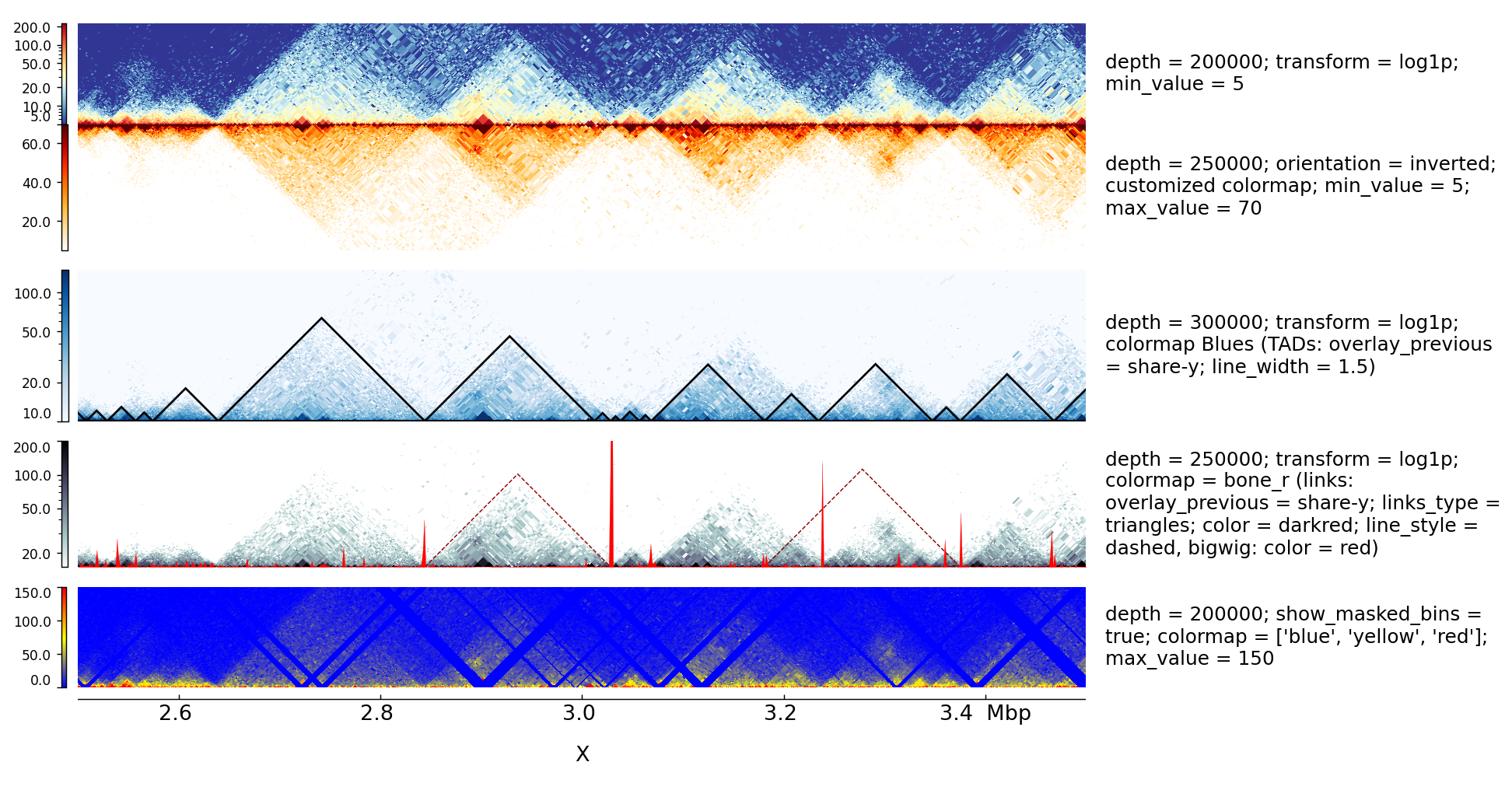
The configuration file for this image is:
[hic matrix]
file = Li_et_al_2015.h5
title = depth = 200000; transform = log1p; min_value = 5
depth = 200000
min_value = 5
transform = log1p
file_type = hic_matrix
show_masked_bins = false

[hic matrix]
file = Li_et_al_2015.h5
title = depth = 250000; orientation = inverted; customized colormap; min_value = 5; max_value = 70
min_value = 5
max_value = 70
depth = 250000
colormap = ['white', (1, 0.88, .66), (1, 0.74, 0.25), (1, 0.5, 0), (1, 0.19, 0), (0.74, 0, 0), (0.35, 0, 0)]
file_type = hic_matrix
show_masked_bins = false
orientation = inverted

[spacer]
height = 0.5

[hic matrix]
file = Li_et_al_2015.h5
title = depth = 300000; transform = log1p; colormap Blues (TADs: overlay_previous = share-y; line_width = 1.5)
colormap = Blues
min_value = 10
max_value = 150
depth = 300000
transform = log1p
file_type = hic_matrix

[tads]
file = tad_classification.bed
#title = TADs color = none; border_color = black
file_type = domains
border_color = black
color = none
height = 5
line_width = 1.5
overlay_previous = share-y
show_data_range = false

[spacer]
height = 0.5

[hic matrix]
file = Li_et_al_2015.h5
title = depth = 250000; transform = log1p; colormap = bone_r (links: overlay_previous = share-y; links_type = triangles; color = darkred; line_style = dashed, bigwig: color = red)
colormap = bone_r
min_value = 15
max_value = 200
depth = 250000
transform = log1p
file_type = hic_matrix
show_masked_bins = false

[test arcs]
file = links2.links
title =
links_type = triangles
line_style = dashed
overlay_previous = share-y
line_width = 0.8
color = darkred
show_data_range = false


[test bigwig]
file = bigwig2_X_2.5e6_3.5e6.bw
color = red
height = 4
title =
overlay_previous = yes
min_value = 0
max_value = 50
show_data_range = false

[spacer]
height = 0.5

[hic matrix]
file = Li_et_al_2015.h5
title = depth = 200000; show_masked_bins = true; colormap = ['blue', 'yellow', 'red']; max_value = 150
depth = 200000
colormap = ['blue', 'yellow', 'red']
max_value = 150
file_type = hic_matrix
show_masked_bins = true

[spacer]
height = 0.1

[x-axis]
$ pyGenomeTracks --tracks browser_tracks_hic.ini --region X:2500000-3500000 --trackLabelFraction 0.23 --width 38 --dpi 130 -o master_plot_hic.png
Log transform and Operation Examples
With the parameter operation you can make operations between one or two files (here two bigwig files but this is also working with two bedgraph files). For example, difference, log ratio, scaling…
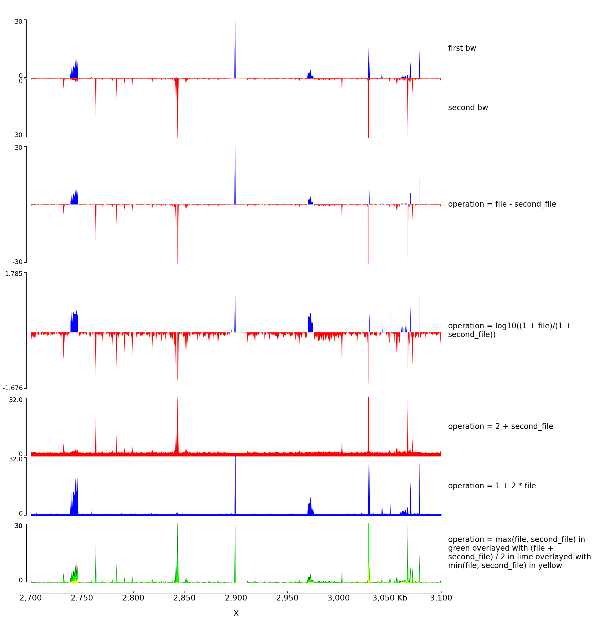
The configuration file for this image is:
[test bigwig1]
file = bigwig_chrx_2e6_5e6.bw
second_file = bigwig2_X_2.5e6_3.5e6.bw
color = blue
height = 4
title = first bw
min_value = 0
max_value = 30

[test bigwig2]
file = bigwig2_X_2.5e6_3.5e6.bw
color = red
height = 4
title = second bw
min_value = 0
max_value = 30
orientation = inverted

[spacer]
height = 0.5

[test bigwig dif]
file = bigwig_chrx_2e6_5e6.bw
second_file = bigwig2_X_2.5e6_3.5e6.bw
color = blue
negative_color = red
height = 8
title = operation = file - second_file
operation = file - second_file
min_value = -30
max_value = 30
nans_to_zeros = true

[spacer]
height = 0.5

[test bigwig op]
file = bigwig_chrx_2e6_5e6.bw
second_file = bigwig2_X_2.5e6_3.5e6.bw
color = blue
negative_color = red
height = 8
title = operation = log10((1 + file)/(1 + second_file))
operation = log10((1 + file)/(1 + second_file))
nans_to_zeros = true

[spacer]
height = 0.5

[test bigwig op2]
file = bigwig_chrx_2e6_5e6.bw
second_file = bigwig2_X_2.5e6_3.5e6.bw
color = red
height = 4
title = operation = 2 + second_file
operation = 2 + second_file
nans_to_zeros = true
max_value = 32
min_value = 0

[test bigwig op2bis]
file = bigwig_chrx_2e6_5e6.bw
second_file = bigwig2_X_2.5e6_3.5e6.bw
color = blue
height = 4
title = operation = 1 + 2 * file
operation = 1 + 2 * file
nans_to_zeros = true
max_value = 32
min_value = 0

[spacer]
height = 0.5

[test bigwig op3]
file = bigwig_chrx_2e6_5e6.bw
second_file = bigwig2_X_2.5e6_3.5e6.bw
color = green
height = 4
title = operation = max(file, second_file) in green overlayed with (file + second_file) / 2 in lime overlayed with min(file, second_file) in yellow
operation = max(file, second_file)
nans_to_zeros = true
max_value = 30
min_value = 0

[test bigwig op4]
file = bigwig_chrx_2e6_5e6.bw
second_file = bigwig2_X_2.5e6_3.5e6.bw
color = lime
operation = (file + second_file) / 2
nans_to_zeros = true
overlay_previous = share-y

[test bigwig op5]
file = bigwig_chrx_2e6_5e6.bw
second_file = bigwig2_X_2.5e6_3.5e6.bw
color = yellow
operation = min(file, second_file)
nans_to_zeros = true
overlay_previous = share-y

[spacer]
height = 0.5


[x-axis]
$ pyGenomeTracks --tracks operation.ini --region X:2700000-3100000 --trackLabelFraction 0.2 --dpi 130 -o master_operation.png
With the parameter transformation you can log transform your data and decide to put on the y axis either the transformed values or the original values:
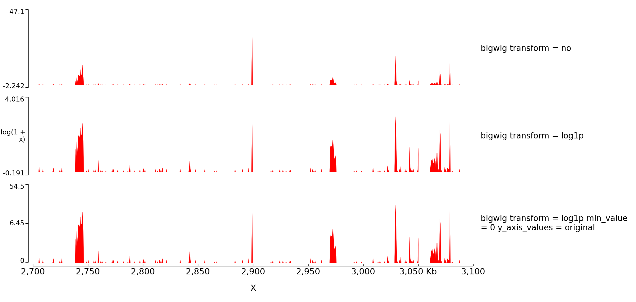
The configuration file for this image is:
[test bigwig]
file = bigwig_chrx_2e6_5e6.bw
color = red
height = 5
transform = no
title = bigwig transform = no

[spacer]

[test bigwig log]
file = bigwig_chrx_2e6_5e6.bw
color = red
height = 5
transform = log1p
title = bigwig transform = log1p

[spacer]

[test bigwig log]
file = bigwig_chrx_2e6_5e6.bw
color = red
min_value = 0
height = 5
transform = log1p
title = bigwig transform = log1p min_value = 0 y_axis_values = original
y_axis_values = original

[x-axis]
$ pyGenomeTracks --tracks log1p.ini --region X:2700000-3100000 --trackLabelFraction 0.2 --dpi 130 -o master_log1p.png
With operation you can also do log transformation however nothing will be written on the left of the y axis:
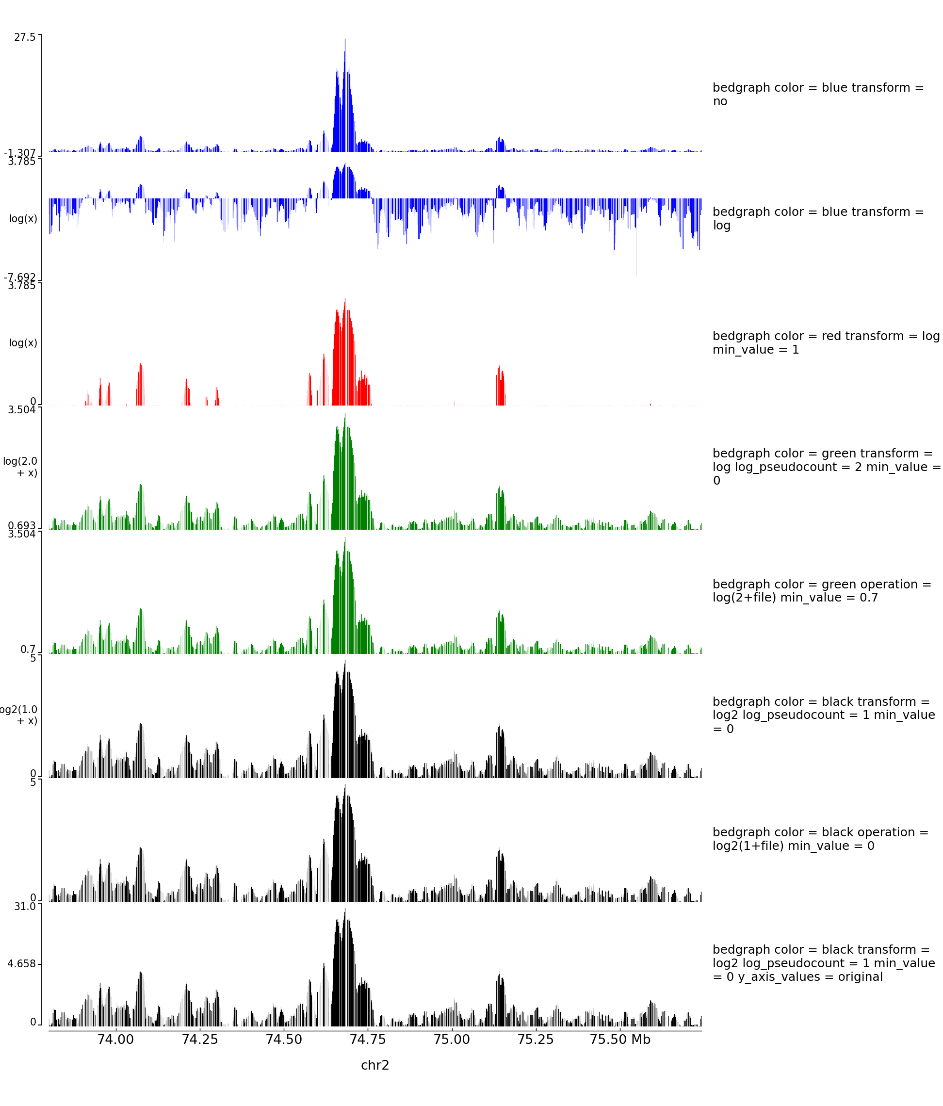
The configuration file for this image is:
[test bedgraph]
file = GSM3182416_E12DHL_WT_Hoxd11vp.bedgraph.gz
color = blue
height = 5
title = bedgraph color = blue transform = no
transform = no

[test bedgraph]
file = GSM3182416_E12DHL_WT_Hoxd11vp.bedgraph.gz
color = blue
height = 5
title = bedgraph color = blue transform = log
transform = log

[test bedgraph]
file = GSM3182416_E12DHL_WT_Hoxd11vp.bedgraph.gz
color = red
height = 5
title = bedgraph color = red transform = log min_value = 1
min_value = 1
transform = log

[test bedgraph]
file = GSM3182416_E12DHL_WT_Hoxd11vp.bedgraph.gz
color = green
height = 5
title = bedgraph color = green transform = log log_pseudocount = 2 min_value = 0
transform = log
log_pseudocount = 2
min_value = 0

[test bedgraph with operation]
file = GSM3182416_E12DHL_WT_Hoxd11vp.bedgraph.gz
color = green
height = 5
title = bedgraph color = green operation = log(2+file) min_value = 0.7
operation = log(2+file)
min_value = 0.7

[test bedgraph]
file = GSM3182416_E12DHL_WT_Hoxd11vp.bedgraph.gz
color = black
height = 5
title = bedgraph color = black transform = log2 log_pseudocount = 1 min_value = 0
transform = log2
log_pseudocount = 1
min_value = 0

[test bedgraph]
file = GSM3182416_E12DHL_WT_Hoxd11vp.bedgraph.gz
color = black
height = 5
title = bedgraph color = black operation = log2(1+file) min_value = 0
operation = log2(1+file)
min_value = 0

[test bedgraph]
file = GSM3182416_E12DHL_WT_Hoxd11vp.bedgraph.gz
color = black
height = 5
title = bedgraph color = black transform = log2 log_pseudocount = 1 min_value = 0 y_axis_values = original
transform = log2
log_pseudocount = 1
min_value = 0
y_axis_values = original

[x-axis]
$ pyGenomeTracks --tracks log.ini --region chr2:73,800,000-75,744,000 --trackLabelFraction 0.2 --width 38 --dpi 130 -o master_log.png